Project: High Angular Resolution Diffusion Imaging Tools
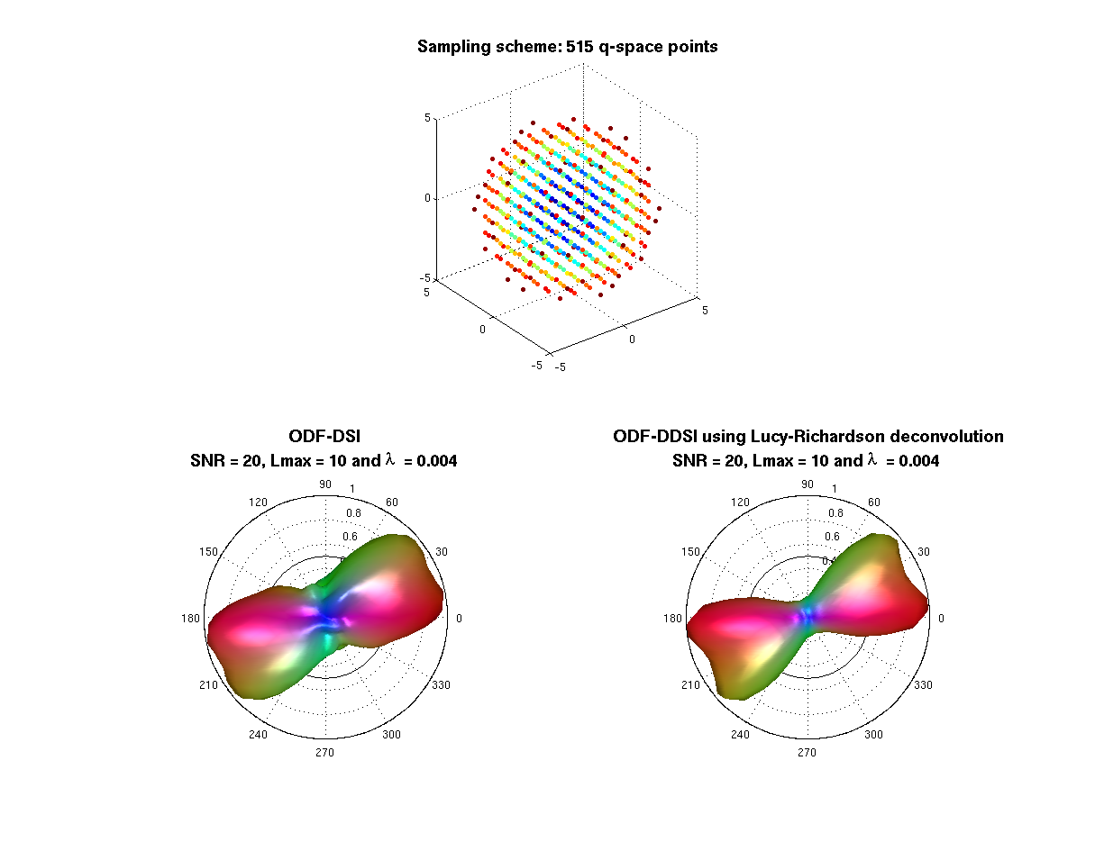
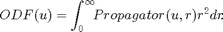
Example to illustrate the Diffusion Spectrum Imaging (DSI) method and the Deconvolved DSI reconstruction. The Orientational Distribution function (ODF) is defined by the radial projection of the propagator computed by the following expression:
The ODF is represented in terms of real spherical harmonic (SH) basis.
- Language: MATLAB(R)
- Author: Erick Canales-Rodríguez, Lester Melie-García, Yasser Iturria-Medina, Yasser Alemán-Gómez
- Date: 2013, Version: 1.2
Contents
- Parameters for reconstruction: All this part is equal for each voxel
clear all; close all; clc;

% - Loading the measurement scheme
%   -------------------------------
% *The gradient_list file represents a keyhole DSI Cartesian acquisition
% to include the set of points in q-space lying on a Cartesian grid within
% a sphere of radius 5, for a total of N = 257 sampling points inside one hemisphere.
% Because of the inherent antipodal symmetry of the diffusion signal. The
% sampling scheme is duplicated on the other hemisphere to obtain the standard 515 points.
% The maximum b-value was 8000 s/mm2.*

gradient_list = load('/sampling_and_reconstruction_schemes/3D_Cartesian_DSI/257_half_with_bvalues.txt');

% Note that the first three columns in gradient_list_257.txt are the unit
% vectors defining the sampling scheme (diffusion gradient directions).
% The last column contains the b-value corresponding to each direction.

grad_red = gradient_list(:,1:3);
bvalues_red =  gradient_list(:,4);

% --- The standard 515 measurement scheme is then:
grad = [0 0 0; grad_red; -grad_red];
bvalues = [0; bvalues_red; bvalues_red];

% --- Transforming the Points to q-sapce
grad_qspace = round(5*grad.*sqrt([bvalues bvalues bvalues]/max(bvalues)));

% - Loading the reconstruction scheme (mesh where the ODF will be reconstructed)
%   ---------------------------------
% unit vectors on the sphere
V = load('/sampling_and_reconstruction_schemes/On_the_sphere/724_shell.txt');
% facets
display(['The reconstruction scheme contains ' num2str(size(V,1)) ' directions']);
F = load('/sampling_and_reconstruction_schemes/On_the_sphere/724_sphere_facets.txt');

% - Defining the parameters for the SH inversion
%   --------------------------------------------
Lmax = 10;
Lreg = 0.004;
display(['The maximum order of the spherical harmonics decomposition is Lmax = ' num2str(Lmax) '.']);
display(['The regularization parameter Lambda is ' num2str(Lreg) ',']);

Laplac2 = [];
for L=0:2:Lmax
    for m=-L:L
        Laplac2 = [Laplac2; (L^2)*(L + 1)^2];
    end
end
Laplac = diag(Laplac2);

basisV = construct_SH_basis (Lmax, V, 2, 'real');
Afix = recon_matrix(basisV,Laplac,Lreg);

% - Defining the parameters for the propagator and ODF computation
%   -------------------------------------------------------------------
Resolution = 35; % The propagator will be computed in a matrix of dimensions: Resolution x Resolution x Resolution
                 % Notice that Resolution is an odd number and so the center of the image is an integer number.
                 % Suggested values for which the PSF computation was optimized are: 33, 35 or 37.

center_of_image = (Resolution-1)/2 + 1;
rmin = 0;
rmax = Resolution - center_of_image;
r = rmin:(rmax/100):rmax; % radial points that will be used for the ODF radial summation
rmatrix = repmat(r,[length(V), 1]);

% --- points that will be used to compute the ODF from the propagator
for m=1:length(V)
    xi(m,:) = center_of_image + r*V(m,2);
    yi(m,:) = center_of_image + r*V(m,1);
    zi(m,:) = center_of_image + r*V(m,3);
end
The reconstruction scheme contains 724 directions
The maximum order of the spherical harmonics decomposition is Lmax = 10.
The regularization parameter Lambda is 0.004,
- Simulated diffusion MRI signal using a multi-tensor model
% --- Experimental parameters
% diffusivities
lambda1 = 1.5*10^-3;% mm^2/s
lambda2 = 0.3*10^-3;% mm^2/s
% S0 is the image at b-value = 0
S0 = 1;
% Signal to noise ratio
SNR = 20;
display(['The signal to noise ratio in this experiment is SNR = ' num2str(SNR) '.']);

% --- Intravoxel properties
% Using a mixture of two fibers (more fibers can be used)
% volume fraction for each fiber (the sum of this elements is 1 by definition)
f1 = 0.5; f2 = 0.5;
% angular orientation corresponding to each fiber (main eigenvector for each diffusion tensor)
anglesF = [0  0;
           45 0];
% [ang1 ang2]: -> ang1 is the rotation in degrees from x to y axis (rotation using the z-axis);
%                 ang2 is the rotation in degrees from the x-y plane to the z axis (rotation using the y axis)
% anglesF(i,:) defines the orientation of the fiber with volume fraction fi.

%  --- Computation of the diffusion signal using the above experimental parameters and intravoxel properties
% *** Signal with realistic rician noise
add_rician_noise = 1;
S = create_signal_multi_tensor(anglesF, [f1  f2],...
    [lambda1, lambda2, lambda2], bvalues, grad, S0, SNR, add_rician_noise);

display ('In this example the true inter-fiber angle is 45 degrees');
display (' ')
The signal to noise ratio in this experiment is SNR = 20.
In this example the true inter-fiber angle is 45 degrees
- DSI and DDSI Reconstruction
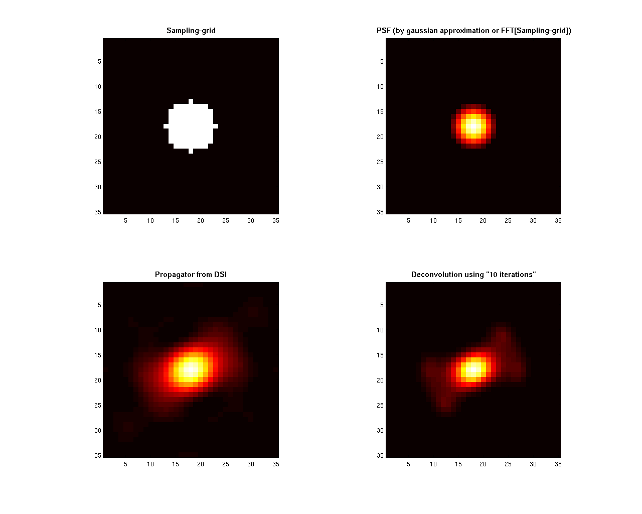
% The noise destroyed the antipodal symmetry of the signal: S(grad) = S(-grad)
% This property can be restored by using the following transformation:
% S(grad) = S(-grad) = sqrt( S(grad)*S(-grad) )

S(2:1+length(bvalues_red)) = sqrt( S(2:1+length(bvalues_red)).*S(2+length(bvalues_red):end) );
S(2+length(bvalues_red):end) = S(2:1+length(bvalues_red));

% --- q-space points centered in the new matrix of dimensions Resolution x Resolution x Resolution
qspace = grad_qspace + center_of_image;

% - Computing the point spread function (PSF) for the deconvolution operation
%   -------------------------------------------------------

%[PSF, Sampling_grid] = create_gaussian_PSF(qspace,Resolution);
[PSF, Sampling_grid] = create_mainlobe_PSF(qspace,Resolution);

% --- Signal in the 3D image
Smatrix = SignalMatrixBuilding(qspace,S,Resolution);
Smatrix = Smatrix/S0;

% --- DSI: PDF computation via fft
Pdsi = real(fftshift(fftn(ifftshift(Smatrix),[Resolution,Resolution,Resolution])));
Pdsi(Pdsi<0)=0;

% --- DDSI reconstruction
% Step#1: Thresholding the resulting propagator
%         (to avoid noise amplification due to the deconvolution)
Pdsi_thr = Pdsi;
SNR_est = 30; % using for example an estimated SNR value
thr = max(Pdsi(:))/SNR_est;
Pdsi_thr(Pdsi_thr<thr) = 0;
Pdsi_thr = Pdsi_thr/sum(Pdsi_thr(:));
% Different stategies may be used to replace this step in real data,
% like thresholding as function of the noise std computed in non-brain voxels,
% wavelet denoising, hanning filtering, etc.

% Step#2:  Lucy-Richardson deconvolution
% Notice that there are some different alternative functions for this
% operation

Niter = 10;
W = zeros(Resolution,Resolution,Resolution);
W(5:end-4,5:end-4,5:end-4) = 1;

% --- option (1): Standard Lucy-Richardson Algorithm: (Implemented in Matlab)
% display('deconvolution "deconvlucy" function');
% Pdsi_lr = deconvlucy(Pdsi_thr, PSF, Niter,sqrt(10^-6), W);

% --- option (2): Standard Lucy-Richardson Algorithm: (Implemented in our lab.)
type_of_noise = 'Gaussian';
%type_of_noise = 'Poisson';
display('deconvolution using "deconv_RL_3D" function');
Pdsi_lr = deconv_RL_3D(Pdsi_thr, PSF, Niter, W, type_of_noise);

% --- option (3): Damped Lucy-Richardson Algorithm: (Implemented in our lab.)
% type_of_noise = 'Gaussian';
%  %type_of_noise = 'Poisson';
% display('deconvolution using "deconv_RLdamp_3D" function');
% Pdsi_lr = deconv_RLdamp_3D(Pdsi_thr, PSF, Niter, W, type_of_noise);

% --- option (4): Lucy-Richardson Algorithm With Total Variation Regularization: (Implemented in our lab.)
%  %type_of_noise = 'Gaussian';
% type_of_noise = 'Poisson';
% display('deconvolution using "deconv_RL_TV_3D" function');
% Pdsi_lr = deconv_RL_TV_3D(Pdsi_thr, PSF, Niter, W, type_of_noise);


% Step#3 Pdsi_lr trilinear interpolation to spherical grid
Pdsi_lr_int = mirt3D_mexinterp(Pdsi_lr,xi,yi,zi);
Pdsi_lr_int(Pdsi_lr_int<0) = 0;
Pdsi_lr_int = Pdsi_lr_int/sum(Pdsi_lr_int(:));

% --- Pdsi trilinear interpolation to spherical grid
Pdsi_int = mirt3D_mexinterp(Pdsi,xi,yi,zi);
Pdsi_int(Pdsi_int<0) = 0;
Pdsi_int = Pdsi_int/sum(Pdsi_int(:));
deconvolution using "deconv_RL_3D" function
- ODF-Reconstruction
% --- Numerical ODF-DDSI reconstruction
ODF_dsi_lr = sum(Pdsi_lr_int.*(rmatrix.^2),2);
ODF_dsi_lr = ODF_dsi_lr/sum(ODF_dsi_lr);

% --- Numerical ODF-DSI reconstruction
ODF_dsi = sum(Pdsi_int.*(rmatrix.^2),2);
ODF_dsi = ODF_dsi/sum(ODF_dsi);

% --- Representing ODF-DDSI in terms of spherical harmonics
sphE_dsi_lr = Afix*ODF_dsi_lr;
ODF_dsi_lr = abs(basisV*sphE_dsi_lr);
ODF_dsi_lr = ODF_dsi_lr/sum(ODF_dsi_lr);

% --- Representing ODF-DSI in terms of spherical harmonics
sphE_dsi = Afix*ODF_dsi;
ODF_dsi = abs(basisV*sphE_dsi);
ODF_dsi = ODF_dsi/sum(ODF_dsi);
- Plots
% --- opengl('software');
feature('UseMesaSoftwareOpenGL',1);

set(gcf, 'color', 'white');
screen_size = get(0, 'ScreenSize');
f1 = figure(1); hold on;
set(f1, 'Position', [0 0 screen_size(3) screen_size(4) ] );
cameramenu;
% -----
subplot(2,2,1:2)
S = 20*ones(size(bvalues));
C = bvalues;
scatter3(grad_qspace(:,1),grad_qspace(:,2),grad_qspace(:,3),S,C,'filled');
axis equal;
title({'\fontsize{14} Sampling scheme: 515 q-space points'},'FontWeight','bold');
% -----
Origen = [0 0 0.25]; % Voxel coordinates [x y z] where the ODF will be displayed
angle = 0:.01:2*pi;
R = ones(1,length(angle));
R1 = R.*f2/f1;
subplot(2,2,3)
polarm(angle,R,'k'); hold on; polarm(angle, R1,'k');
% the ODF is scaled only for the display
plot_ODF(ODF_dsi./max(ODF_dsi), V, F, Origen);
title({'\fontsize{14} ODF-DSI ';...
       ['SNR = ' num2str(SNR) ', Lmax = ' num2str(Lmax) ' and {\lambda}  = ' num2str(Lreg)]},'FontWeight','bold');
axis equal; axis off;
% -----
subplot(2,2,4)
polarm(angle,R,'k'); hold on; polarm(angle, R1,'k');
% the ODF is scaled only for the display
plot_ODF(ODF_dsi_lr./max(ODF_dsi_lr),V, F, Origen);
title({'\fontsize{14} ODF-DDSI using Lucy-Richardson deconvolution';...
       ['SNR = ' num2str(SNR) ', Lmax = ' num2str(Lmax) ' and {\lambda}  = ' num2str(Lreg)]},'FontWeight','bold');
axis equal; axis off;
% -----
display (' ')
display ('Notice that the deconvolution operation increases the resolving power of the method')

% -----
f2 = figure(2); hold on
set(f2, 'Position', [0 0 screen_size(3) screen_size(4) ] );
set(gcf, 'color', 'white');
screen_size = get(0, 'ScreenSize');

colormap hot
subplot(2,2,1)
imagesc(Sampling_grid(:,:,center_of_image));
title('\fontsize{11} Sampling-grid','FontWeight','bold');
axis square

subplot(2,2,2)
imagesc(PSF(:,:,center_of_image));
title('\fontsize{11} PSF (by gaussian approximation or FFT[Sampling-grid])','FontWeight','bold');
axis square

subplot(2,2,3)
imagesc(rot90(Pdsi(:,:,center_of_image),3));
title('\fontsize{11} Propagator from DSI','FontWeight','bold')
axis square

subplot(2,2,4)
imagesc(rot90(Pdsi_lr(:,:,center_of_image),3));
title (['\fontsize{11} Deconvolution using "' num2str(Niter) ' iterations"'],'FontWeight','bold')
axis square
Notice that the deconvolution operation increases the resolving power of the method