Project: High Angular Resolution Diffusion Imaging Tools

Example to illustrate the Spherical Deconvolution reconstruction via the Lucy-Richardson (L-R) algorithm. The fiber ODF is defined by the multi-tensor diffusion model.

Language: MATLAB(R)
Author: Erick Canales-Rodríguez, Lester Melie-García, Yasser Iturria-Medina, Yasser Alemán-Gómez
Date: 2013, Version: 1.2

- Parameters for reconstruction: All this part is equal for each voxel
- Simulated diffusion MRI signal using a multi-tensor model
- Initial estimate of the S0 component from the signal
- fODF estimation via the standard and damped L-R algorithms
- fODF estimation via non-negative least squares
- Plots

- Parameters for reconstruction: All this part is equal for each voxel

clear all; close all; clc;

% - Loading the measurement scheme

grad = load('/sampling_and_reconstruction_schemes/On_the_sphere/70_shell.txt');
% grad is a Nx3 matrix where grad(i,:) = [xi yi zi] and sqrt(xi^2 + yi^2 + zi^2) == 1 (unit vectors).
display(['The measurement scheme contains ' num2str(size(grad,1)) ' directions']);

% - Loading the reconstruction scheme (mesh where the fiber ODF will be reconstructed)
%   ---------------------------------
% unit vectors on the sphere
disp(' ')
V = load('/sampling_and_reconstruction_schemes/On_the_sphere/724_shell.txt');
% facets
display(['The reconstruction scheme contains ' num2str(size(V,1)) ' directions']);
F = load('/sampling_and_reconstruction_schemes/On_the_sphere/724_sphere_facets.txt');
disp(' ');

% - Creating the Kernel for the reconstruction.
%   ---------------------------------
% Kernel is a Dictionary of diffusion tensor signals oriented along several
% directions on the sphere (in our example V, which is the set of orientations where the fODF
% will be computed).
% It also includes two compartments with isotropic diffusion to fit real Brain data: CSF and GM

% diffusivities assumed for the Dictionary
lambda1 = 1.2*10^-3;% mm^2/s
lambda2 = 0.0*10^-3;% mm^2/s (Like the ball and stick model of T. Behrens)
% b-value and grad: equal to the experimental parameters used to adquire the data
b = 3*10^3;% s/mm^2
grad = [0 0 0; grad]; % Add a measurement with b-value = 0 into the gradient matrix
                      % (standard format in which the signal is measured in the scanner)

SNR = 20; % This is a parameter required for the "create_signal_multi_tensor" function,
          % however, in this case the signal will be generated without noise.
add_rician_noise = 0;

[phi, theta] = cart2sph(V(:,1),V(:,2),V(:,3)); % set of directions
Kernel = zeros(length(grad),length(V) );
S0 = 1; % The Dictionary is created under the assumption S0 = 1;
fi = 1; % volume fraction
for i=1:length(phi)
    anglesFi = [phi(i), theta(i)]*(180/pi); % in degrees
    Kernel(:,i) = create_signal_multi_tensor(anglesFi, fi, [lambda1, lambda2, lambda2], ...
                                             b, grad, S0, SNR, add_rician_noise);
end
% adding the isotropic compartment for CSF
lambda1 = 2.0*10^-3;% mm^2/s
Kernel(:,length(phi) + 1) = create_signal_multi_tensor([0 0], fi, [lambda1, lambda1, lambda1], ...
                                             b, grad, S0, SNR, add_rician_noise);
% adding the isotropic compartment for GM
lambda1 = 0.7*10^-3;% mm^2/s
Kernel(:,length(phi) + 2) = create_signal_multi_tensor([0 0], fi, [lambda1, lambda1, lambda1], ...
                                             b, grad, S0, SNR, add_rician_noise);
%   ---------------------------------

The measurement scheme contains 70 directions
 
The reconstruction scheme contains 724 directions

- Simulated diffusion MRI signal using a multi-tensor model

% --- Experimental parameters --- %
% new real diffusivities
lambda1 = 1.5*10^-3;% mm^2/s
lambda2 = 0.3*10^-3;% mm^2/s
% S0 is the image at b-value = 0
S0 = 100;
% Signal to noise ratio
SNR = 20;
display(['The signal to noise ratio in this experiment is SNR = ' num2str(SNR) '.']);

% --- Intravoxel properties --- %
% Using a mixture of two fibers (more fibers can be used)
% volume fraction for each fiber (the sum of this elemenst is 1 by definition)
f1 = 0.5; f2 = 0.5;
% angular orientation corresponding to each fiber (main eigenvector for each diffusion tensor)
anglesF = [0  0;
           55 0];
% [ang1 ang2]: -> ang1 is the rotation in degrees from x to y axis (rotation using the z-axis);
%                 ang2 is the rotation in degrees from the x-y plane to the z axis (rotation using the y axis)
% anglesF(i,:) defines the orientation of the fiber with volume fraction fi.

%  --- Computation of the diffusion signal using the above experimental parameters and intravoxel properties %
% *** Signal with realistic rician noise
add_rician_noise = 1;
S = create_signal_multi_tensor(anglesF, [f1  f2],...
    [lambda1, lambda2, lambda2], b, grad, S0, SNR, add_rician_noise);

The signal to noise ratio in this experiment is SNR = 20.

- Initial estimate of the S0 component from the signal

% --- find zeros
grad_sum = sum(abs(grad),2);
ind_0 = find( grad_sum == 0);
S0_est = mean(S(ind_0));

- fODF estimation via the standard and damped L-R algorithms

% --- parameters definition
%type_of_noise = 'Gaussian'; % (Default reconstruction published by Flavio Dell’Acqua!)
type_of_noise = 'Poisson'; % (Experimental, not extensively tested, it provides sharper solutions)
Niter = 200; % optimal value between 200 and 400 (for Gaussian noise)

% -- Initial solution: Constant value on the sphere, non-negative iso-probable spherical function
fODF0 = ones(size(Kernel,2));
fODF0 = fODF0/sum(fODF0);

% --- standard L-R reconstruction
display(' ')
display('This is the real/effective time required for computing the fODF at each voxel')
display(' via the standard L-R algorithm:')
%
tic
[fODF_std, fgm1, fcsf1] = sph_deconv_RL(S/S0_est, Kernel, fODF0, Niter, type_of_noise);
% fgm is the fraction of the isotropic component in GM tissues.
% fcsf is the fraction of the isotropic component in CSF.
toc

% --- damped L-R reconstruction
display(' ')
display('This is the real/effective time required for computing the fODF at each voxel')
display(' via the damped L-R algorithm:')
%
tic
[fODF_d, fgm2, fcsf2] = sph_deconv_RLdamp(S/S0_est, Kernel, fODF0, Niter, type_of_noise);
% fgm is the fraction of the isotropic component in GM tissues.
% fcsf is the fraction of the isotropic component in CSF.
toc

 
This is the real/effective time required for computing the fODF at each voxel
 via the standard L-R algorithm:
Elapsed time is 0.027782 seconds.
 
This is the real/effective time required for computing the fODF at each voxel
 via the damped L-R algorithm:
Elapsed time is 0.069130 seconds.

- fODF estimation via non-negative least squares

display(' ')
display('This is the real/effective time required for computing the fODF at each voxel')
display(' via the linear least squares algorithm with nonnegativity constraints:')
%
options = optimset('lsqnonneg');
options = optimset(options,'TolX',1e-14);
tic
fODF_pos = lsqnonneg(Kernel, S/S0_est,options);
fgm3  = fODF_pos(end);       % fraction of the isotropic component for GM
fcsf3 = fODF_pos(end-1);     % fraction of the isotropic component for CSF
fODF_pos(end-1:end) = [];    % purely anisotropic part
toc

 
This is the real/effective time required for computing the fODF at each voxel
 via the linear least squares algorithm with nonnegativity constraints:
Elapsed time is 0.024180 seconds.

- Plots

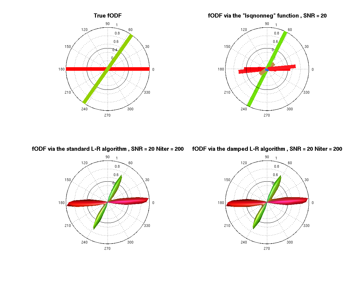
% --- opengl('software');
feature('UseMesaSoftwareOpenGL',1);

set(gcf, 'color', 'white');
screen_size = get(0, 'ScreenSize');
f1 = figure(1); hold on;
set(f1, 'Position', [0 0 screen_size(3) screen_size(4) ] );
cameramenu;
title('Spherical deconvolution methods')
% -----
Origen = [0 0 0.25]; % Voxel coordinates [x y z] where the ODF will be displayed
angle = 0:.01:2*pi;
R = ones(1,length(angle));
R1 = R.*f2/f1;

subplot(2,2,1)
polarm(angle,R,'k'); hold on; polarm(angle, R1,'k');
% ---
anglesF = anglesF*(pi/180);
[Vx, Vy, Vz] = sph2cart(anglesF(:,1), anglesF(:,2), ones(size(anglesF,1),1));
for i=1:size(Vx,1)
    hold on
    Color_i = [Vx(i) Vy(i) Vz(i)]/sqrt( Vx(i)^2 + Vy(i)^2  + Vz(i)^2 );
    Color_i = Color_i.*sign(Color_i);
    line([-Vx(i) Vx(i)], [-Vy(i) Vy(i)], [-Vz(i) Vz(i)], 'LineWidth', 10, 'Color', Color_i);
end
% ---
title('\fontsize{14} True fODF', 'FontWeight','bold')
axis equal; axis off;

subplot(2,2,2)
polarm(angle,R,'k'); hold on; polarm(angle, R1,'k');
% ---
% the fODF is scaled only for the display
fODF_pos = fODF_pos./max(fODF_pos);
ind0 = find(fODF_pos == 0);
fODF_pos(ind0) = [];
Vaux = V; Vaux(ind0,:) = [];
Vx = Vaux(:,1); Vy = Vaux(:,2); Vz = Vaux(:,3);
for i=1:size(Vx,1)
    hold on
    Color_i = [Vx(i) Vy(i) Vz(i)]/sqrt( Vx(i)^2 + Vy(i)^2  + Vz(i)^2 );
    Color_i = Color_i.*sign(Color_i);
    line(fODF_pos(i)*[-Vx(i) Vx(i)], fODF_pos(i)*[-Vy(i) Vy(i)], fODF_pos(i)*[-Vz(i) Vz(i)], 'LineWidth', 10, 'Color', Color_i);
end
% ---
title(['\fontsize{14} fODF via the "lsqnonneg" function , SNR = ' num2str(SNR) ], 'FontWeight','bold')
axis equal; axis off;

subplot(2,2,3)
polarm(angle,R,'k'); hold on; polarm(angle, R1,'k');
% the fODF is scaled only for the display
plot_ODF(fODF_std./max(fODF_std), V, F, Origen);
title(['\fontsize{14} fODF via the standard L-R algorithm , SNR = ' num2str(SNR), ' Niter = ' num2str(Niter) ], 'FontWeight','bold')
axis equal; axis off;

subplot(2,2,4)
polarm(angle,R,'k'); hold on; polarm(angle, R1,'k');
% the fODF is scaled only for the display
plot_ODF(fODF_d./max(fODF_d),V, F, Origen);
title(['\fontsize{14} fODF via the damped L-R algorithm , SNR = ' num2str(SNR), ' Niter = ' num2str(Niter) ], 'FontWeight','bold')
axis equal; axis off;

Project: High Angular Resolution Diffusion Imaging Tools

Contents

- Parameters for reconstruction: All this part is equal for each voxel

- Simulated diffusion MRI signal using a multi-tensor model

- Initial estimate of the S0 component from the signal

- fODF estimation via the standard and damped L-R algorithms

- fODF estimation via non-negative least squares

- Plots